Saturday, 18 May 2013

Knapsack 0/1 problem and algorithm: Implementation in Python, Dynamic programming and Memoization

This post is on the Knapsack algorithm which does the following. You have a list of items each with a value and weight. You have a total capacity as limit. You have to take as many items to increase value within the limit. A good example, similar to the one given by MIT Professor John Guttag (in open courseware) is, you break into a bank vault with a sack which can hold 100Kg of weight. You are faced with a pile of gold coins,  million dollar bonds, a huge stack of Marlboro cigarettes, stacks of red bull and Heineken. How much of each should you take  given your limit? A better example is you are going to Mars and your allotment in the shuttle is 400Kg and you have to take items that are valuable in that limit.

The Algorithm is recursive but, uses memoization to cut short the search through the solution tree. i.e for a pair (number of things remaining to take from, remaining capacity) i.e you have 5 more things to take from and weight limit is now 30Kg then, what do you take for this? If this is already solved in the recursion somewhere we use that, instead going down to that. This is where memoization comes in and Python dictionary is well suited for this. So, you have sub problems and find optimal solutions to those problems and solve the parent problem.

The result of the algorithm is a pair (V, I) where V is the accrued value of items we decided to take. I is the list of items we decided to take.

Knapsack 0/1 Algorithm Pseudo code:

knapsack(<L: list of items>, <W: weight limit now>, <S: solutions accumulated over sub-problems so far>)
{
        IF S is empty i.e first call THEN
           Initialize S the set/dictionary to hold solutions to sub-problems

       IF  combination of (L, W) is already in S THEN
           (V,I) for this sub-problem =  S(L, W)
       ELSE IF L is empty and W is 0 THEN
           (V, I) is (0, nothing)    
       ELSE IF we take the first item on list and its weight, when added, exceeds the limit THEN
              (V,I) = knapsack(L - first item at this call, W, S)
       ELSE
               /* What we do here is. We assume we take the first item. Then what is (V,I) for the remaining
                   walks. Also, what is the result (V,I) id we don't take the item at this point. Choose which
                   ever solution that maximises the value.
               */
               We assume we take the first item of the list.
                Let V1 = Value of first item + (V, I) for knapsack(L - first item, W - weight of first Item, S)
                We also find (V2, I) if we don't take the item.
                       i.e (V2, I) for knapsack(L - first item, W, S)
             
                IF V1 is better than V2 THEN
                       go with that result (V1, I)
                ELSE
                       go with the other result (V2, I)
       Add the corresponding result (V, I) to S
}

Sample with the following items. <Item Name, Weight, Value>

('Gold Biscuits', 20, 100)
('Heineken', 2, 30)
('Marlboro', 1, 10)
('Currency in $10 bills', 10, 10)
('Currency in 50$ bills', 45, 40)
('Million$ Govt Bonds', 1, 1000)
('Diamonds', 25, 80)
('Lays Chips', 1, 4)
('RedBull Cans', 20, 35)
('Predictions on WallStreet', 1, 200)
('Key Combination of Vault', 1, 200)
('Harry Potters List of real life Spells', 2, 1)

Sample Output: As you can see the program takes the things of value :))


Solution Python Code: Is available at
https://drive.google.com/folderview?id=0BxhHg0qy5gi4TkpuTHQ4OWZGYnc&usp=sharing

References:

1. MIT Open courseware on Introduction to Computer Science and Programming, Prof John Guttag

Monday, 13 May 2013

Quick Sort: Partition Algorithm

A post on quick sort is not particularly interesting for most developers. But, when you see more and more people using a complicated partitioning algorithm when explaining quick sort then, it is ok post a simpler partitioning algorithm. This algorithm and similar ones came in the Communications of the ACM and were retold by Bentley in his books. Still, they seem to be lost.
 
Quicksort works recursively by partitioning an array around a pivot element. So, after partitioning all the elements at indices less than the pivot's will be less the pivot itself. Those at indices greater than the pivot's index will be greater. Then, you repeat the same for elements on either side of the pivot. For example, if the array was 4, 19, 1, 3, 43, 45, 11, 2 and you say that, the pivot is 4 then, after partition around element 4, the array looks like this using this partition algorithm (explained further down).

2, 1, 3, 4, 43, 45, 11, 19

Then do quick sort on (2, 1, 3) 4 (43, 45, 11, 19). You get the idea.

So now comes the simpler partitioning algorithm. Here starting from the beginning
we keep track of elements greater than the pivot and whenever we see an element less than the pivot we replace the element which is greater than the pivot (we have it) with the one that is lesser.

So in our example if 4 was the pivot, 19 is the first element that is greater than the pivot, we go on to 1 and see that it is less than the pivot. We swap the two to get 4, 1, 19, 3, 43, 45, 11, 2. Now also we keep track of (index of) the first element that is greater than pivot. Again, we swap it for 3 and the array becomes 4, 1, 3, 19, 43, 45, 11, 2. Then, finally we meet 2 and then swap it for 19 and the array becomes 4, 1, 3, 2, 43, 45, 11, 19. So we have reached the end of the array. Our post condition is that, the pivot should be in such an index that, all elements to the left are less and those to the right are greater. This is achieved by simply swapping the pivot with our track index (here the index of 2). So we swap 4 and 2. Thus we get 2, 1, 3, 4, 43, 45, 11, 19.

Here is a snap of the partition code.
You can run the code in debug mode and see for yourself as to how this works.

The eclipse java project is available at theGoogle docs folder given below.

https://drive.google.com/folderview?id=0BxhHg0qy5gi4V2Q0ZlhrelZlOVU&usp=sharing

Tuesday, 7 May 2013

Google AppEngine: The network is becoming the computer

This post is a take on the Google AppEngine which is a cloud computing solution living in the Platform As a Service (PaaS) layer. A basic sample code is available at the end but, more concrete examples of this post are available on the resources mentioned in the reference section below.

Google AppEngine is Google's, to some extent free, web app execution environment for you. You can develop web applications and deploy it on AppEngine in an instant. You production execution environment is the offer. Traditionally, you design a webapp, the pages, middle tier and the database etc. You also have to install software for your production environment. With AppEngine, you just write the code and upload it. It will be available immediately on Google's infrastructure which you don't have to spend time and money on. On top of it all, is the ability to scale, replicate like Google.

In order to use AppEngine, you just need to signup on the AppEngine site with a email and password. If you have a Google account it is enough. The main applications that are suitable for AppEngine are the ones that require to talk to an HTTP(s) endpoint. Basically, web based applications like an online forum. You are restricted from doing traditional stuff like creating local files, opening outgoing sockets etc. But, you do have a lot of overwhelming options to add to your site like, email, instant messaging, distributed filesystem API, Memory caching, my favorite. You can develop using Python 2.7 which is what I used and also using Java, Google Go with corresponding SDKs from Google. There are number of web frameworks supported including Django. Here I followed the very basic webapp. 

If you have done servlet based development then, it is easy to get first hold of AppEngine. As always you have an application configuration file similar to web.xml. Here it is a .yaml file. My project's yaml file is shown below

You specify the script which will handle the requests to your server url. This script can be thought of as a controller servlet in Java Web programming using servlets. Then with in that python code, you create the application, specify the url mappings, the classes to handle the url mapping requests and you are basically done. So, in helloworld.py, I have the following similar to an MVC web app.

Also the code for the main handler as below, which has get and post to handle the request like servlets.

Set up on Ubuntu Linux:
1) Download the AppEngine Python sdk from Google. This is a zip file.
2) Extract it to say, /usr/local/appengine-python
3) Create links to appcfg.py and dev_appserver.py file in the above path at /usr/local/bin. So that, you can run these programs. This can be done using the command

 sudo ln -s /usr/local/google_appengine/appcfg.py /usr/local/bin/
4) Your folder /usr/local/bin will look something like this
5) Download the Eclipse plugin for AppEngine development and you are done. Although this is not necessary unless you use eclipse.

Uploading your project to AppEngine
1) Go to the root of you webapp project and execute the command as shown below. You will be asked a email and password for authentication and then your app will be provisioned instantly. You can access it at http://<appid when you created it on Appengine site>.appspot.com

2) The site on Google AppEngine
3) Download code for the project from link:
https://drive.google.com/folderview?id=0BxhHg0qy5gi4SFh6ejhBSFE2ZU0&usp=sharing

More explanations on code and features in next post.

Reference:
--------------
1) Core Python Applications Programming Chapter 12 on Google AppEngine.

Monday, 6 May 2013

Part 2 - Friend Suggestion like Facebook, Google+ or Product Suggestion like Amazon: Implementing for your own web app, site

In a previous post in the first half of 2012, I described how to roughly do a friend suggestion like Google or Facebook or item suggestion like Amazon. I am recalling the approach in that post before describing how to use machine learning to get better results. 

In the previous approach, we used to store vectors of user interaction on the hadoop file system. These vectors may include interaction between users or with the site. There we used MapReduce jobs to derive some meaning of the interactions and then using a weighted matrix to apply thresholds and priorities to arrive at the final result.

One thing that, I did not mention in that post is the use of machine learning libraries which have algorithms that can help in such scenarios. For example, Amazon uses machine learning techniques to show you Product recommendations. The counts we described in the previous post are crude although not completely off the chart. This is also used (in addition to proprietary algorithms, Facebook is coming up with a Graph search and algorithms on top of that could possibly make this easy) by Facebook / Linkedin to suggest 'you may know this person' type of recommendations. The focus of this post is that, we should use machine learning libraries to process interaction patterns and arrive at results. 

Input: We imagine that, we have large logs of user interactions, user likes (Facebook), Following items (Google plus) etc at some place on a Hadoop cluster. The best thing would be to use HBase as it is column oriented and is supposedly used at Facebook. Some examples can be user viewed another profile, user likes a movie, user viewed a video of a particular type, user changed his home town. All sorts of interactions. Labels and tags are used to aid this (remember the tags on videos in YouTube and labels on blogger posts!). 

Basically for every interaction or relation we can call it a dimension. For example, viewing another users profile is a dimension. Likes on movies is a dimension. Watching a video of a particular type say 'of Lady Gaga' is a vector in a dimension. Once we have these interaction vectors, we can find what is the affinity of the user in that dimension or type. A good place to start for finding affinity is the percentage frequency count or better the percentage frequency in a particular time period, the latter being more relevant. For example by using MapReduce on the interaction logs on Hadoop, we can arrive at numbers saying that, for the last day userA watched 4 videos tagged with 'Lady Gaga' and viewed profiles of 20 users in Washington D.C area. Such vectors are easy to generate. Refer the 'Hadoop Definitive guide' Tom White's book which has examples similar to this on earthquake data for the US. In a way you don't need to store as logs, you can directly feed the interaction vectors to HBase since it is column oriented ! But, you still need to derive a basic meaning out of the interactions before feeding them to machine learning.

Machine learning can be used to classify, cluster and some other stuff too. Here we are interested in these. Item Recommendations, Clustering and User Neighborhoods are a good place to start when you want to analyse user behavior. Clustering is useful when you want an overall view across all dimensions/vectors we discussed. So, the vectors from the MapReduce jobs are fed to machine learning which gives you results like userA is in neighborhood of userB, userA may like  itemC since he/she is in the same neighborhood as userB, in movies/movie likes dimension userA is similar to userB etc. You can refer to 'Mahout in Action By Sean Owen' on how to get going with this. Sample code in Chapters will be helpful. 

So all together the new approach looks similar to the case studies mentioned in Tom White's book.

Logs /HBase data -> Map Reduce -> Machine Learning -> Recommendations -> Store to RDBMS for provisioning. 

This seems a better way for item recommendations and the like compared to the previous post. More ways on how to this are available online. 

References
--------------
https://www.youtube.com/watch?v=kI4YIYInou0
https://www.youtube.com/watch?v=9A0PnPvQks4
Hadoop the definitive guide - Tom White (Book & code)
Mahout in Action - Sean Owen and team (Book)

Monday, 8 April 2013

Programming for Social Media : Twitter : Reading Tweets using python

Just to bring the aspect of search, social media into perspective before the post: 

Todays ACM technews has an article from Eberly College of Science relating to tweets analysis relating to a particular vaccine. It is available at 
http://science.psu.edu/news-and-events/2013-news/Salathe4-2013 Tweets were analysed for terms relating to the vaccine/vaccination. Then, user opinion was deduced. This is an example of using social media to derive trends or responses or acceptance.

As another example of impact of internet search: Earlier in December, during an informal Big Data meetup involving, Ministry of Health, Visa and SingTel, the head of MoH software division commented that, Google could find out if, there would be an outbreak of a particular disease say a flu in a particular region. This is due to the fact that, people would be searching for medicines, symptoms, prevention etc on Google. This could be analyzed to deduce what health issues are more prevalent in a particular region. 

Thinking on that line, Google does not know if, you actually bought the medicine or anything after a search. Whereas Amazon or eBay knows what you bought but, does not know if, you bought the item after a search or your affinity for that item. Standing out is Facebook which knows everything about you and your friends but, does not have the above two factors.

That said here is a small program that, demonstrates Python Twitter API. This retrieves tweets on an interesting subject and processes them. The tags in each tweet are counted and displayed in ascending order. For example, if #Tottenham appears 20 times and  #OldTrafford appears 40 times in the tweet stream, then it comes up in the list. Basically, a measure of what people are dicussing and how popular the topic is with the public.

Objective: Retrieve tweets with "premierleague" on it. Then find the most popular tags. Basically you can search for any key word.

Language used Python 2.7 and Twython for Twitter interface. Operating system Ubuntu 12.04. 

Twython API core code snapshot for Twitter


Sample Screen run on keyword "premierleague". (Printing tag counts by minute rather than by hour so that, output is available frequently)


The complete eclipse python project is available here as zip. You will need a postgresql database and Twython installed. The database table format is available here. You can also run TaTwitterQn/TwitterSearcher.py without the database to get tweets and show the tag counts.

Project Link:
https://docs.google.com/file/d/0B-oeIeog2xb7WDRFLUdzM0w0cEE/edit?usp=sharing

Some Issues/observations developing this program: https://github.com/ryanmcgrath/twython/tree/master/core_examples

1) Tweepy a popular Twitter API for python returns an 401 failure for search / filter operations. This is on the latest version of Tweepy from Git. But, tweepy has streaming api.

2) python-twitter seems to be a good api but, does not authenticate at times and also some of the documented parts do not seem to work. For example, the getHashTags part of the Tweets API does not work.

3) The same program can be coded in Java but, the effort would be more and the code size too. Python on the other hands was small and easy. If you already have a Java environment like Hadoop running then, it seems ok.

References:
1) https://github.com/ryanmcgrath/twython/tree/master/core_examples This is a good list of examples to use twython and you can get started to do your own programs easily.

Sunday, 31 March 2013

ANTLR 4.0

If you do use Google Analytics, you may have noticed that, the API is available for developers to use. Also, on a Youtube video showing "Google Analytics End to End", the engineers show 2 ways that developers can interact with Google Analytics. One is through an API that Google has exposed for developers to use. The second is a small edit box where you can type in the metrics / filters and you click on a button and you get the results based on the filters you mentioned.

Typing things in an English like question / expression which is not exactly sql but, will get you the results you are looking for does come in handy especially since, ordinary users can interface with your system easily. This is conceptually same as the Interactive Shop Finder in malls except that, you type in the question you are looking for. Users will be able to relate to this kind of interface as they will be able to test drive your software. 

Considering that, you need to cook up an expression / question that you will take from the user, parse that and get the results; means you need a small language that will allow your users to express themselves. This may have you filters as pre-defined keywords. For example, ga.City = Pasadena and ga.Country = USA is similar to what Google gives you. 

ANother Tool for Language Recognition will allow you to specify the Backus Naur Form of your small language and build you a parser. So all you have to do is;

u
1) Use ANTLR to specify the BNF of your small language
2) Get the parser for your language using ANTLR.
3) Use the parser to parse the user question
4) Catch the elements in the question that makes sense to you. i.e walk the expression tree. This is possible by assigning labels to your grammar rules. This is extremely helpful when you are walking the tree.
5) Build the real query that your database takes and get the result.


References:

ANTLR website has a lot of examples, and the BNF of the mainstream languages like Java and the like. So developers can hit the ground running designing their own small languages.

Sunday, 23 December 2012

Data Analytics : Hatari !

Embedding Pig in Python - Hatari!
---------------------------------------------
Pig Latin does not allow control structures like Java and other high-level languages. So inorder to get more control over the execution context, loop through a set of parameters etc we can embedd Pig in Python. This is supported only for Python 2.7 and not above. At first this may seem not so useful. But, if you have a single script, i.e a parameterised pig script like the one in the previous post, you can attach parameters to the script from Python. Plus since Python can also be used to write User Defined Functions, all the code Pig, Python, UDFs reside in the same project. This is usefull when things get more complex. In the previous post note that, I used a java project to create a java UDF which was used in Pig. So I had 2 deployments a pig script and a Java jar. But, if we embedd pig in python, we have only one deployment, the python code.

1) Write pig script in a file.
2) Use compileFromFile() function to load and compile your script. 
3) Bind using your list of map of parameters. yes a list of map of parameters.
4) Run the script using runSingle()
5) Get status on how things went using runSingle(). You can also use isSuccessFul().

Better yet Do this again for all your scripts. You can even read parameters from a file, add threading where each thread will execute a script with one set of parameters.

Source code with an example is available here

Ref: More details can be found in the presentation at http://www.slideshare.net/julienledem/presentation-pig-scripting by Julien Le Dem.

Ref: Good Read Chapter 9 on Book, Programming Pig by Alan F Gates

Data Analytics: Using Apache Pig User Defined Functions

Apache pig helps to analyse large data sets. We can define data flows in pig latin scripts and extract interesting information from the initial data set. For example, we may have a large data dump of user actions on your website as a csv file or in a database like hbase. Then we want to find the most frequented part of your site or the top 10 things that interests your user base in your site. To write up a solution for this is possible in a highlevel language like Java. The optimizations for handling data size as it grows, splitting the task into multiple parts, keeping track of those individual tasks will be challenging and will consume a lot of effort. Apache Hadoop and Pig help to solve this problem by providing a framework with which we can focus on the data flow rather than on the plumbing.

Derieving interesting data is always tied to a time period. We may want to extract interesting information from the whole life time of the data or we want to perform the same on a given time period say the last month or week. To specify such options, we have user defined functions in pig. This allows us to write filters and operations that we want pig to perform on each entry of the data set. This gives more control on the data filtering, flow. Some of the nuances of pig udf are explained in the example below.

Pig Version of this example: Apache Pig version 0.10.0 (r1328203)

Objective: You want to write a filter function in PIG to filter data rows according to a date range that you are interested in. You want to invoke the script from a scheduler which passes in the date range as command line parameters. A pig script is shown in the image below.


1) Passing command line parameters to pig script: You need to pass command line arguments like this pig -param datefrom='2012-10-20 00:00:00' -param dateto='2012-10-23 00:00:00' -x mapreduce user-based-analytics.pig. (I am actually calling the script from Python, which we will see in the next post).

Here I am using these two date parameters to build my Java UDF. If you are passing parameters with space character, it has to be like this otherwise pig will throw an error saying that, it cannot create your UDF java class.

2) With in the pig script: You refer to the command line parameters using the format '$' for example, '$dateto' and '$datefrom' as in the image above. unless it is an integer like $parallelism.

3) Defining your UDF reference using DEFINE pig keyword: This allows you to create a reference to your UDF which you can call using an alias. For example, the script defines a reference to the UDF as follows,

define date-based-filter com.home.pig.udfs.TimeStampFilter('$datefrom', '$dateto')

where date-based-filter is the alias that I will use to call my UDF com.home.pig.udfs.TimeStampFilter java class.

4) Calling your UDF filter in a pig script using FILTER keyword: Pig does not have a boolean data type. But, expressions are evaluated to boolean true or false. You need to call your UDF as follows, with the alias for your UDF. Here we are checking for datebasedfilter(ts) == TRUE i.e does my UDF 'com.home.pig.udfs.TimeStampFilter' acting on the current row with 'dateto' and 'datefrom' return Java Boolean true or false.

filter-by-date = filter site-data by date-based-filter(ts) == TRUE;

5) Now the Java Class that does the filtering.

a) We have to create a java class that extends FilterFunc from org.apache.pig.FilterFunc. The constructor has to take parameters that, you set in the script above. So we have two parameters.

b) Override the public Boolean exec(Tuple arg0) member function to define how this filter will handle tuples from the script. Here I just get the date from the string and check if it is within the range.

c) Package this in a jar and put it in the same location path as your script.

Why use Pig and UDF
s? Writing UDFs can be easy and saves a lot of time compared to writing a MapReduce Java program or any other option. Plus, if you have a ton of data or will end up with one this is better option since Hadoop will scale and Pig will do the jobs like data groupings, filtering for you.

Better to use Python? Although it is easy to write the UDF in Java and the justification that Pig is in Java, there is already a java environment turned on; it may be better to write User Defined Functions in Python and also trigger the script in for greater control! plus every thing will be at one place.

For more on this topic Refer to Chapter 10 in Book, Programming Pig by Alan F Gates

Thursday, 16 August 2012

Go Parallel

Objective : To Parallelise merge sort algorithm.

The part of merge sort that presents opportunity for parallel programming is the merge part. This takes two sorted arrays and merges them. The usual algorithm compares each element of the two arrays and writes them in order and finally writing the array with more elements, if any. 

For parallel merging there is another algorithm, for two arrays A and B. Choose an element X of A so that it divides A into two almost equal parts A1 and A2. Find where X will fit into B (using binary search). Split B at this point into B1 and B2. Merge A1 and B, A2 and B2 recursively. The advantage is that, these two merges can be implemented by independant hardware such a multiple processors since the loop dependancy of the serial algorithm is removed in the parallel algorithm. The program will provide a visible speed up on Cilk plus for intel. But, on Java vm on my 2 core processor machine the speed up is overrun with the overhead for scheduling, Executor service in Java concurrency package.

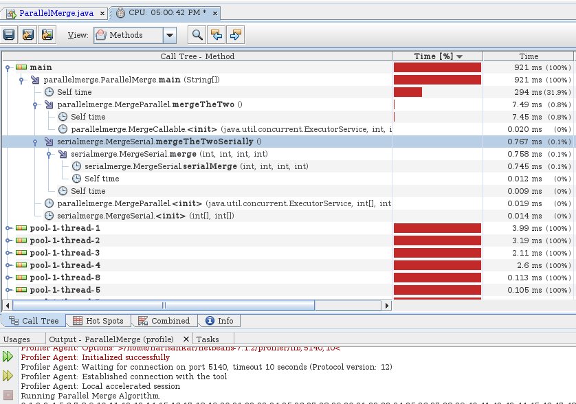
The run times of parallel and serial merges are shown below. The overhead of Future, Callable, Executor in java concurrency package is coupled with the recursive calls.

The parallel merge is 10 times slower with two cores But, it is up to the jvm to parallelise. In Java, programmers use concurrency package for parallel executions whereas C++ has a number of opensource options for targeting multi core parallelism. The speedup approaches  serial speeds depending on the judicious choice of when to stop the recurssion tree (ie the number of elements at which we switch to serial merge!).

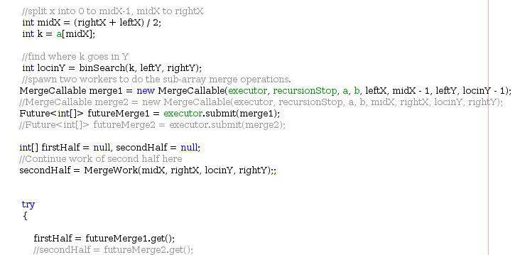
The Java code part spawns a new thread for one of the merges described above and the calling thread continues with the current merge. We can use two threads for each of the sub-merges but, it adds to the overhead. The first approach is shown below with the latter commented.
This is a fork and join approach/pattern for parallel programming. We can also use a map pattern for parallel programming by dividing the array conveniently and merging at multiple stages using a reducer, maybe that will give a lot more direct speed up than fork-join pattern.

Reference: This technique for parallel merge sort originally appearing in 'Structured Parallel Programming' from Morgan Kaufman. If interested read this book.

Monday, 16 July 2012

Living with Linux Desktops: KDE4 V Xfce on Opensuse 12.1

Here is a brief comparison of Xfce desktop and KDE desktop that comes with opensuse linux 12.1. The screen shots for the konsole using top command for memory and system monitor shows the difference. Notable is that KDE Dolphin uses 25MB whereas, Thunar the default file browser for Xfce used 17MB. Half of Dolphin. On CPU and memory Xfce desktop has half resource usage compared to KDE4. I have not used KDE plasma graphics too much on my desktop. KDE4 desktop is configured to use clean looks and use suse look and feel. Having Xfce on an older hardware can make it faster or comparable to a new hardware running latest operating system. 

File Manager
----------------
Dolphin 25MB
Thunar 17MB

Comparison
----------------
          CPU(2cores)      Memory
KDE      6, 3.9%                      0.30 GB / 2.0 GB
Xfce     2, 3.9%                      0.16GB / 2.0 GB

Xfce feels responsive and faster. In fact too fast. The one disadvantage of Xfce is that, sometimes the widgets/panel apps don't work. For example, the window manager had to be started manually at command line. Or the windows did not have close/minimize/maximize buttons. Again, Lock Screen does not seem to invoke any response from Xfce and also resuming after hibernating does not prompt for password by default.

Screens

KDE Top and System Monitor

Xfce Top and System Monitor

Monday, 9 July 2012

Friend Suggestion like Facebook, Google+ or Product Suggestion like Amazon: Implementing for your own web app, site

This is an application of Apache Hadoop MapReduce framework. Facebook has a feature that says that, some people may be your friends. This is calculated based on a number of factors such as common friends, likes, visits to profile,
comments made etc. Basically the interactions is logged, analyzed and put through a kind of weighted matrix analysis and the connections which are above a threshold value are chosen to be shown to the user.

Problem: An input file of 1GB size with the logs of interactions among 26,849 people. To keep the data manageable on my computer, I am creating random logs with interaction of 1000 people with the rest of the people on the, say social
networking site. Gathering and presenting this data to map reduce is itself a job. In our case, these 1000 people need friend suggestions.

Solution: Here this is done in a Single map reduce job although, more data and intermediate jobs can be added in real life. The mapper for the job takes each interaction and emits the user pair and interaction statistics. For example,
Sam Worthington has 1 profile view, 2 friends in common, 3 likes with Stuart Little. so the out put of the mapper here is . We could use the userid across the site rather than a name. For each person interacting with Stuart Little a record like this is produced.

The reducer simply takes the output of the mapper and calculates the sum of the interactions per user-user pair. So, for a week of interactions the record from the reducer may be, for example, . This is got by summing up the interactions by the reducer. Then, each interaction can be given a weight/value then, the number in the record can be multiplied by the weight and summed. Any calculation is ok as long as it give a meaning result based on the interaction types. Then, interactions with a score larger than a threshold can be chosen to be presented to the user when they login.

Other factors like user interests, activities etc can also be accounted for. Here we can simple treat each as a user and emit a record if there is a related activity in user's profile and proceed as usual. The same approach can be applied to ad serving utilizing info from user profile and activity. A Combiner and mutiple jobs can be used to get more details too.

Results: For 1GB, in real life big data approaches > 2TB, of randomly generated log of interactions of 26K+ people with a select 1000, the mapreduce program gave the friend suggestions in 13 mintues on my laptop with a pseudo distributed Hadoop configuration. So, if you have a few tera bytes of data and 10 computers in a cluster you can get the result in say 1.5 hours. Then all that is needed would be to consume the friend suggestions via a regular db / webservice and present it to the user when they log in.

Screen shots of the Map Reduce job run on pseudo distributed Hadoop:

1) Copying the data to Hadoop Distributed File System


2) Running the jobs

3) Status on Hadoop admin interface.

4) Friend Suggestions with statistics.


5) Job code

6) Mapper

7) Reducer

Sunday, 1 July 2012

Apache Hadoop Map Reduce - 1

Hadoop is a map reduce framework that allows for parallel distributed computing. The criteria for adopting Hadoop is that, the same operations are performed on records and records are not modified once created. So Reads are more frequent than write in a traditional relational database system. The advantage of Hadoop or a Map Reduce frame work comes into action when the data is large enough ~ 1TB. Above this point data is referred to as big data approaching PetaB. At such a point it is better to throw multiple machines at the task rather than to use a single machine with parallel programming. The technique used is Map Reduce which deals with Key and value pairs.

A map operation is performed on records whose inputs and outputs are key value pairs themselves. The output is merged, sorted and submitted to a reduce operation which combines and generates the output. For example, we have 12 years of student records for examinations across 15 subjects. The total number of records is 5,700,000. On this data set we can find operations such as highest score on a subject over the years, total failure reported across the year etc. To find the total failures, the map operation outputs a key value pair   every time it encounters a failed exam. The reduce job takes all such key value pairs and emits a Key value pair .

The hadoop standalone configuration on these records finished in ~ 35-40 seconds. The hadoop run start is shown here
 The run end is here
Output is here. 

The same on a pseudo clustered mode gives results for similar operations in ~40 seconds. The difference is that, the input files have to copied into the Hadoop distributed file system and the output needs to be copied/read from the HDFS. As shown here

Saturday, 2 June 2012

Java Concurrency - Beyond Synchronized


Synchronized keyword is frequently used in Java. But, Synchronized cannot provide a method for threads to signal one another of conditions that others may be waiting on. Another thing is that synchronized does not act on a fairness policy. A thread that is starved for quite some time need not get access over others. i.e the fact that you have been waiting for some time may not be considered. 

An example for conditions is availability of elements in a shared data structure queue. Such a facility is provided by java.util.concurrent.locks.Condition. This allows threads to wait for a condition on a lock and relinquish the lock so that, other threads can full fill the condition that is needed for the waiting threads to continue. This logic can be programmed using locks but, Condition provides this off the shelf. Once the lock is acquired thread waits for the condition mandatory for it to continue. When the condition is true it continues. 

Fairness policy is allowed by a Reentrant lock where the thread waiting for quite sometime will get access. 
The intriguing part of threading in Java is that, the time (in ms) between a consumer / producer is able to regain access to a shared data structure is the same with Condition as it is without Condition. 

Example: Producers & consumers waiting on a lock & its condition. Both share a common queue where the producers put in integers for the consumers to take, contending for the queue access at the same time.  

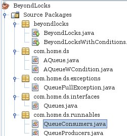
Code Structure

Code with Synchronized keyword.

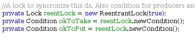
Condition creation code.

Code with Condition.

The consumer comes back on receiving the signal

Monday, 14 May 2012

Facade Pattern - Java Code Architecture

Object oriented programming involves instances of classes i.e objects interacting with one another towards a common goal. This interaction can be for services, control or data. Objects perform a particular function in a software. When there are a lot of objects the code becomes cumbersome to maintain and use; every time in the same piece of software. 

Facade pattern comes into action when you have a subsystem that performs a particular service for another subsystem or part of the code. A subsystem here in terms of software code means a group of objects interacting to get a job done. Facade pattern hides the objects underneath it and their interactions to object layers above the pattern. For example, information collected from the user interface in a java application may be used to create say, a user object, account object and the user interface may store this to the database by using an object that performs that database operation. Here a Facade object can expose an operation, i.e creating the objects from the data from UI and storing it to the database. This facade can be used by the UI without delving into the details of how it is done. 

If the interaction of the objects in the facade changes, it is contained within the facade and no layer of code outside the facade is affected. This is the most important aspect of the facade pattern that makes it so useful in Java Enterprise where this pattern is more frequently seen in popular Java Enterprise IDE's ready-made-code.

For example, suppose there is a table in the database that stores the details of attendees in a conference. Java enterprise wraps this with an Entity say, Attendee entity which would be part of the JPA ready-made-code. This entity will expose the database operations on the table. A facade would be created namely a session facade which exposes operations that are utilised by controller layers to update information.  The session facade will deal with the requests on the Attendee Entity. 

Here is an example of the code structure for a Tomcat based application that gets information in a table. Called from a servlet. i.e servlet is the controller in Model-View-Controller Application model. 

as you can see from this code, the facade is called to do the job. The code to get a job done becomes small as far a controller object is concerned. A lot of things may happen under the facade but, the higher layer object does not care about this. It is the Facade's responsibility. The code structure in eclipse web project is shown below. There are entity objects and Facade objects. Facade objects here share a common ancestor which declares common operations on entity-facades. In this example, entity objects simulate the JPA entity objects.


The abstract facade is not a must in the general facade pattern but, is used here as is further simplifies code with inheritance. A part of abstract facade is shown here 
A subclass of this called Attendee Facade used in our example is here 
A lot of object interactions and code is thus abstracted from a controller object / higher level object by using the Facade Pattern. It also makes the code more reusable, maintainable, predictable and beautiful.

Thursday, 5 April 2012

Skip Lists Algorithm and Runtime Profiling

Skip List Runtime on dictionay operation compared to Splay Trees and Hash Tables. (Coded in Java)

Skip lists are a relatively new data structure. This is an ordered list where the nodes are connected together at multiple levels. Different levels of connected nodes need not be uniform. This allows the skip list to skip items during a search. Each level is an ordered list in itself.  Every node has a level and is connected to different nodes in the same level. This allows data structure operations to skip through the list. Example is the following list where there are two levels.

Level 1 connections                  E ----------> X
Level 0 connections A ->; B -> E -> F -> G->X -> Y -> Z

Level 0 list is the same as a linked list. E has connections has two levels. If a search was for say 'G'. The algorithms is as follows Start at Level 1, X > F so we move down at 'E' and then proceed at level 0 from E till G is found. Nodes A and B were skipped.

SkipList Search Algorithm:
1) Start from the top level proceed until level 0
    a) Move to the right until a node with node Key < search Key
    b) Jump to the next lower level.
2)  If 1a resulted in an exit in level 0, the next node could be the search node. else it is absent.

Here is a skip list implementation holding values A to Z. The nodes encountered during the search for H and M are shown.

Level 2 Skip List. 


Level 6 Skip List
In order for the list to be helpful level at each node needs to be decided at Random during the insert operation of that node. The maximum level that is useful in a skip list is ln N -1 where N is the number of items expected to go into the skip list. 

Algorithm Inserting in to the Skip List

1 Find the node as in search. This will return the node that will be to the left of the new node (L).
   a) While dropping down to the lower levels maintain the nodes in an update List.
2 Create the new node with a random level. 
3 Adjust the pointers from the existing L node to the new node.If the new level is greater than the existing level of the list, then the head of the list should be adjusted to point to the new node at the new level.
4 Set the next pointers of the new node to next pointers of L
5 Set next pointers of L to the new node at that level. This is done for each node where level was changed in step 1.

For example in the case of 
Level 1 connections                  E ----------> X
Level 0 connections A -> B -> E -> G->X -> Y -> Z. We need to insert H with level 3 then, at level 1 we drop down at E and also at G in level 0. So, G->next = H at level 0, E-> next = H at level 1, F -> next = X at level 1 and at level 2 H is linked to head and tail of the list.


Level 2 connections                                  *<-H->*
Level 1 connections                  E ----------->H-> X
Level 0 connections A -> B -> E -> F -> G->H->X -> Y -> Z

Runtime of Skip Lists: Dictionary operations on skip lists take O(Log(n)) time. Finding each new node's level is done in random as follows


Comparison of Skip List, Splay Binary Search Trees and Hash Table

For a serious input of 56000 word dictionary, the search operations on Skip lists, Splay Trees and Hash Table is as follows. Skip list took 40 comparisons at 11 levels to find the word 'Skip' in the dictionary.


Splay tree took less time than the skip list at
Hash Table left the above two way behind in run time

Result: In general skip lists and splay trees can't hold candle to hash tables.