Australia Tax Stats 2011-12 | Visualisation & Insights

This post visualises Australian Tax data for Individuals during the income year 2011-12. This web application allows the user to explore tax filing data to derive a number of insights. The data is available from the Australia Government website here. 

Watch the video for a look at this application. 

Specific Insights
============

1) Size of the workforce has not changed much: If the Wikipedia page on Australian economy is correct, then the workforce has not changed from 2011-12. The workforce count on the data confirms this.

2) Workforce made up of Equal numbers from both genders: Tax data shows that almost the same number of men and women figure in the filings.

3) State-wise gender gap in registered salary: Data shows that women, when compared to men, although roughly the same number in the workforce as men have their cumulative salary field at half the $ number in WA. This gap varies for the states. Since the number of women is almost the same, this wage gap triggers cause-analysis such as:

1. Women are paid less in the same job compared to men.
2. If (1) is not true then, women are not in the same pay band/scale or jobs as men are in. This would explain why the salary is less even though women make up the same head count.

4) Taxable Income/Salaries for under 18 age and above 70: The data shows that there is healthy income (but < 1 Billion) for these two age groups.

5) Comparison of states: On all accounts the ranking is NSW, Victoria, Queensland, WA, SA, TAS and other.

There are other data points like child support by filing individual, refundable, exemptions etc which can be analysed.

Data visualisation: Plotting USGS earthquakes

This post makes use of USGS's live feed of earthquakes. The feed is plotted on a Leaflet map to visualize the data. Leaflet is a javascript library for interactive maps (http://leafletjs.com/). The advantage is that it consumes Geojson well.  

Feeds are categorised into all quakes and significant ones. The app's hourly feed is updated continuously for new data. When new data is available the map is updated. For each point of interest a leaflet layer group is utilised. This holds a circular marker layer and a place holder. A popup layer is also added which displays a text with the title from geojson. This title includes magnitude and location of the quake. All layer groups are added to the map's layer group. This allows individual layers associated with a point to be update or removed when data is updated.

Although all earth quakes are not significant, from the data is clear that earthquakes are more common in plate boundaries and fault lines (not surprising but nice to visualise). Switching to a weekly or monthly view makes vulnerable locations apparent.

Significant quakes are also seen in daily, weekly and monthly basis. Adding filters to query on Magnitude or changing the circle marker circumference based on magnitude would be good. However, significant earthquakes are far less in number and are shown separately in the app. Also to be noted is that, leaflet slowed down when a lot of layers were used for each point to support individual point updates. It also eases out when the map is just cleared and updates are added.

Tools:

Python 3.5.3
Django 1.10
Postgresql
Bootstrap 3.3.7
Leaflet 1.2.0
Javascript, JQuery
Geojson

Building a recommendation engine for Dota2

This post builds a recommendation engine that suggests heroes for a Dota2 player. This was one in a 3 set requirements to be completed. For more about Dota2 read on wikipedia and this. Two other requirements include player comparison and a leader board.

The application that was built looks like this.

Requirement: Dota2 has a set of 113 heroes and a huge community of players. The requirement was to suggest a hero for a given player. The recommendation engine should take into account play history of the specific player and heroes. Dota2 open API documentation is available at https://docs.opendota.com/ and the application must use this as a source of data for recommendations. The API for the solution must be available as REST and also on a web page. 

Approach: The solution is built as a collaborative item-to-item recommender. The data set for training and building the recommender is available from this api. An example for this api call to dota2 looks like this https://api.opendota.com/api/players/87568060/heroes?date=30 The result of this query has the hero play history (30 days back) for the player with id 87568060. For a list of players this can be utilised to build a data set. The advantage of using this api query is that it fits the recommender well as it has the play history for the heroes (by the players). And by using the data for all the players it contributes to the collaborative nature of the recommender. The resulting data set has the following columns and rows for each player to hero game plays.

player_id -> steam id for a player  

hero_id  -> id of the hero

plays -> number of times that this player played the hero.

This information is used to build a co-occurence matrix of all heroes to the player's heroes. This matrix is normalised using Jaccard index and a sorted weighted sum is applied to get the list of recommendations. Dota2 open api allows only 3 requests per second. So memcached is used to cache results of the external dota2 api call. The data set is divided into training and test respectively. The matrix is built on the training data. The matrix is built as follows

The disadvantage of this approach is that there needs to be a play history in place. Otherwise the matrix would be zero. This is the same for a new hero. One approach is to suggest a set of easy to play heroes to beginners. Again, this implementation builds the matrix for a subset of the players or for the whole community. The first case can be modified to build the matrix for only play history of beginners which would take into account hero plays of other beginners (collaborative).

Tools used:

Python 3.5.3

Django 1.10 & Django REST Framework

Pandas 0.20.3

Postgresql 9.5

Memcached

AWS EC2
Bootstrap

Reference:

For a good basic introduction to recommender systems see
https://www.youtube.com/watch?v=39vJRxIPSxw

Django models: I will cache you if I can

This post presents a generalised approach to making cache keys for Django model from fields and related one-to-one fields. In the last post  a Django model based approach to cache keys was utilised. However, that results in code duplication for the purpose of generating cache keys. At first look that appears inevitable since each model is cached in its own way. However as more requirements come in, a pattern can be identified and code duplication can be avoided. This new approach to making cache keys is enabled by a base class that inherits from models.Model and provides mechanisms to generate keys. The cache key generation takes into account what model fields the key has to be based on. 

For example, if there is a Player model with fields id, email, username. We may want a cache key that would look like 'model.used.id.<the_id>'. Same for email and username. However, what if many fields of a model need to be in the cache key? This post presents a solution. Again, what if there is a one-to-one model which has a foreign key back to Player and that model needs to be cached ? For example, consider a model PlayerStats with fields id, user, stats. When this model needs to be queried it is likely to be based on the user. So, it makes sense to have a cache key for PlayerStats based on its linked player. Since this approach takes in any field, this becomes easy. The base class is

The class methods give back the cache key template and the instance method generates the cache key for the instance. The template is needed when some model's fields+values are available and we need to check the cache for those. Example is a web request asking for User with id=10 and we want to check that if that user is in cache.

The Player model will inherit from CacheableModel,

The PlayerStats looks like this

Now all that remains is a utility that takes in Model classes and calls the two class/instance methods.

- Now when Player needs to be queried on id, say from a Django view it becomes as easy as.

model_ins_from_cache_by_fields(Player, {'id': steamid})

- For Player stats for a specific player, this becomes

player = model_ins_from_cache_by_fields(Player, {'id': steamid})
player_totals = model_ins_from_cache_by_fields(PlayerTotals, {'player': player})

That is saving a lot of "if in cache else" code from repeating in views.

Some things to keep in mind:

1) Notice that the __str__ of the models is used for building keys. So make sure that __str__ of models do not have spaces and control characters.

2) Since it is based on __str__, if the __str__ represention is too long then the cache key becomes too long, possibly to the extent of increasing the time of hashing for the key.

Both these are addressable and is left as homework for reader. ;-)

Tuning the word cloud: Nuances with Mobile-support/REST-api/Cache

The word cloud web application in the previous post has been updated with the following features.

1) Mobile/Tablet support using Bootstrap css.
2) Configurable ignore lists to reduce noise in the cloud.
3) Caching.
4) REST.

1)  Mobile/Tablet support

Bootstrap makes the app usable on various device screens. Bootstrap intro page here. A page from the application now looks like this.

2) Ignore list via Configuration 

A web page can now be set with a list of words to ignore. There is no point so far in counting the word "like" on a social media page. Now the application can have words associated with lists and those lists associated with a web page. i.e configurable ignore lists. Example.

After applying an ignore list there is visible reduction in noise. (before Vs after).

3) Caching

This is most challenging in any application. When the data has not changed in the db, time spent on db/disk accesses for the same can be saved thus improving app latency. Memcached is used on 2 hosts and the application is configured to use the same. When a page is requested, data access is first checked against the cache, if it is a miss then only the db is queried. This data from the db is cached right away so that subsequent requests for the same data return fast. Common challenges in caching is described below. It is important to develop a feature without caching and then put the caching logic in. Screens show cache hits/miss on 2 consecutive requests for the same data. The second request returns from cache hits.

 

 

4) REST API

Data needs to be provisioned in a way that can be consumed by mobile applications, web apps or any program that wants to talk to your application. REST is good especially for native mobile applications that need the data but, handle display on their own. Django REST makes this manageable with a few quirks of its own. A rest response from the application using Chrome is shown and the same is accessible using curl command too.

  
The rest of the post is about common programming challenges in DRF and caching.

DRF challenge

DRF is good at so many levels. However it is tightly couple with the queryset. So if there is a list of instances rather than a queryset, things become incompatible. For example, customizing a foreign key related field to use cached data before hitting the database. While this may be a remote requirement the problem is well explained here. Curiously, Django1.10 has a new feature that lets queryset api with instances list. This api feature is described here. So if the instances that match are already in the cache they can be used. DRF serializer can be made to work with model instances like

The eager loading idea is from here but has been modified for the specific requirement with instances. After this what remains is overriding the get_queryset on the rest view. Works with Django 1.10. If the api is heavily used and database accesses can be saved, it is worth the effort and work too.

Caching Challenges

 

1) What to cache? 

To avoid access to the database, it is common to cache database entries. Images, static pages and json responses are also cached.

 

2) Cache code: 

Where to put it? How generalized should it be? Good cache key? In tutorials it is common to see cache access code and if that fails the object is retrieved from db and set to cache. This is leads to a lot of duplication of code. It is better to identify common sql access patterns to the db and cache those. The code that caches the db can be set as a behavior of the database entity or coded as a utility. Example for cache access logic as part of the db entity facade/ORM. This orm approach is described here.

Modify that for reuse: common accesses like the above on primary key can be factored out for re-use in a utility module.

Some access types are difficult to generalize and doing so can make the code base difficult to maintain. For example, fetching an entry in table A that corresponds to a foreign key. While it may be tempting (and feasible) to make a utility for this too, it is better to leave this alone until replication makes the use-cases clear and creates a demand for factoring this out into a utility.

  

What works in terms of generalizing the cache code depends on how many requirements come up. After a number of use cases, a general pattern should emerge in any application, like the primary key and foreign key access above.

 

3) Cache Key? 

A good cache key is one which describes the cached content. Also it should not be so long that the time to compute the hash beats the whole purpose.

 

4) Cache invalidation? 

If the data that is cached has changed then the cache needs to be updated. If the data is updated at many points in the application, it may become difficult to keep track of this. The example shows a signal handler that updates the cache on a db update/save. This approach works well.

 

5) Cache loading

Finally, when the application starts up, it is good to have the cache initiated with some data. What qualifies to be loaded to cache on startup? A fixed number of entries/tables with fixed row count or most frequented data points make good candidates. The application data, UI and usage need to be analyzed to determine the same. For example, data that corresponds to drop down lists with fixed number of entries. Say the names of states in a country shown in a drop down list.

Word clouds: Text analysis for interesting patterns

This post utilises text analysis to identify trends in popular web pages. Of interest are home pages of news sites, Twitter pages of popular personalities and other sites where content changes frequently. Analysing words and projecting to a cloud provides a visual representation of text data which in turn helps to quickly perceive overall changes in trends and interests. Here the cloud is generated on content from Saturday and Sunday.

About the application:

The web application generates a word cloud for each submitted link at a given time. The application first generates a word count for each page using natural language tool kit and stores the results in a database. The counts are converted to a word cloud using opensource javascript libraries. Web links can be added to the application as needed. The word count task is performed asynchronously using celery worker nodes. 

Software built using:

Django1.10/Python3.5, Asynchronous tasks using Celery 4.1.0, Javascript, Natural Language Processing Tool Kit (NLTK), Postgres Database. 3 hosts. One for web application, one for celery workers and Database and third for the message broker. 

Home pages analysed:

RT.com
BBC.com
Google News
Fox News
Indian Prime Minister Twitter Page
Obama Twitter page
President Trump Twitter Page

Celery Django Architecture

>> Word cloud on Saturday to left and Sunday to right

RT.com
BBC.com
Fox News
Google News
Obama

 President Trump and  the Indian Prime Minister Twitter Handles

Band-aid for profiling in a hurry

This post profiles two solutions to a problem to see which one has low latency. As it will be obvious the better solution employs a simple technique and requires no explicit confirmation that it returns faster. Quickly profiling does not hurt either.

The objective is to consecutively calculate the n-th fibonacci where each n is taken from a sequence. Solution 1 is a recursive algorithm. This divides the problem into sub-problems and builds the final solution by combining solutions to individual sub-problems. This solution does not make any other attempts at gaining faster speeds. Solution 2 is also recursive but, uses a map to hold the results of sub-problems encountered during the calculation. That way for each subsequent n in the sequence, the results of sub-problems from the previous run are re-used. The same can be achieved with memoization.

As seen in the profiling results Solution 2 not only saves execution cycles but also saves itself from the overhead of context switching into the sub-problems.

Solution 1 without state

Solution 2 (with state in a class)

Now we profile the two solutions by calculating over a list of 10 numbers and the results are shown below.

Results

Sharded database on a MongoDB cluster

MongoDB is a NoSQL document store. As with other NoSQL databases there are a number of advantages to it including dynamic schema, scalability/performance and no need for ORM layer. A production deployment of MongoDb should be clustered. This will increase scalability and durability for the data. For high volume applications the number of disk operations and network transfers can overwhelm a single node. Example is any back-end for mobile apps with millions of users. On a single node memory is also a precious resource that can become scarce. Finally the whole data set can be too large to fit in one node or one set of nodes. Sharding helps to address these issues. 

This post shows the setup of a sharded cluster and checking the behavior when the primary in a replicaset fails.

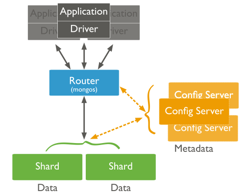
A sharded MongoDB topology looks like the following.

There are at least 3 config servers, 1 router and then the shards themselves. Each shard should ideally include at least 3 nodes/servers. One of the nodes in the shard will be elected primary and data replicates to the others in a shard. There can be many shards depending on data set size. The router routes a query to a particular shard after consulting the config servers. So on a minimum there needs to be 7 hosts for a basic sharded cluster. These have to be separate and not vms on the same machine. If these are vms on a single big server in production then we are not addressing the issues that led to the move towards sharding. However the post used vms all on ssd. The setup is described as below.

Setup details

Build 7 vms or configure separate hosts (recommended) with the following. Either an available image can be used or clone using virtualbox.

Config server

192.168.56.30

192.168.56.31

192.168.56.32

Shard's data nodes

192.168.56.40

192.168.56.41

192.168.56.42

Router

192.168.56.20

Each node runs on 64-bit Ubuntu Server 16.04 and uses MongoDB 3.4.1.

Database used is the MoT dataset from https://data.gov.uk/dataset/anonymised_mot_test

Config servers

A) Start the config servers one by one. Log into the config server and run the following command.

mongod --configsvr --replSet config_set1 --dbpath ~/mongo-data --port 27019

In the version of MongoDB used the config servers themselves are a replicaset. mongo-data is the path for storing the data files. Do this for each config server.

Log into one of the config servers in mongo and initialise them as shown:

Shard nodes

B)  On each node in the shard start the mongo daemon as

mongod --shardsvr --dbpath ./mongo-data/ --replSet data_rs_1

Log into one of the data nodes and initialise them as shown

Router

C) Start the router. On the router node 

mongos --configdb config_set1/192.168.56.30:27019,192.168.56.31:27019,192.168.56.32:27019

Adding shards

D) Connect to the router and add the shard to the cluster.

View the config server to confirm that the shard was added. This shows up in the SHARDING logs.

Shard the database

E) Enable sharding for the database and collection in that order. Again connect to the router to do the following.

mongo> sh.enableSharding("mot")

Then enable sharding for the collection. Also specify the key field that needs to be used for distributing the data between shards.

F) Check the shard status. On the router do a sh.status(). This should look like

Verify

G) Connect a client to the router and populate the database. After this the shard status also shows chunks of data.

H) Check the config on the cluster. Connect MongoDB Compass to the router and look into the config db.

Note that an index is created on the DB for the shard key. This is shown below.

Electing a primary on failure:

Setting the above up can be time consuming but it is all worth it as when the primary node of the shard is killed, one of the other data nodes assumes the primary position through an election. So we go and kill the primary node process. This result in heart beat failure and after waiting for a specific time frame one of the secondaries assumes primary position. This is shown below.

The primary was node 192.168.56.40.

On failure of that 192.168.56.42 is elected as primary. This shows up on the 40 node when it comes back online.

Although queries during primary election can fail it can be caught in exceptions and tired again in the application. This requires no mentioning but the daemons should be run as service.

Reference:

MongoDB docs at

https://docs.mongodb.com/manual/tutorial/deploy-shard-cluster/

This can be a bit outdated but is a good read too
https://www.digitalocean.com/community/tutorials/how-to-create-a-sharded-cluster-in-mongodb-using-an-ubuntu-12-04-vps